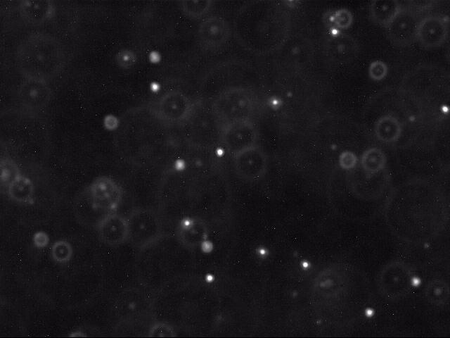
 An individual frame showing the polystyrene beads illuminated against a backdrop of water
The final project for Princeton University’s Intro to Computer Science course involves providing an estimate for Avogadro’s Constant (6.02 x 10²³) using a scientific method involving the analysis of Brownian motion. All code for the project can be found on the repo.
At its core, the estimation comes from gathering data from recorded footage of polystyrene beads undergoing Brownian motion in water. The change in position for each bead within each video experiment can be fitted to the Stokes-Einstein relation. Four Java files were needed to translate that data into a single estimation for Avogadro’s constant:
Blob.java: Representation of a set of light pixels (connected or unconnected) defined as a complete set representing a polystyrene “blob”. Has a defined mass and center of mass coordinates in the x-y plane.
BeadFinder.java: Designates a blob of a minimum designated number of pixels as a “bead”. Takes in a picture containing blobs and determines which blobs can be considered beads using a recursive depth-first search algorithm. This filters out all extraneous light in each frame of the video to track the actual polystyrene beads in question.
BeadTracker.java: Tracks beads and their movement from one frame of a video to the next. Prints the distance change (radial displacement) of each bead after each frame change.
Avogadro.java: Calculates a self diffusion constant which is then used to approximate the Boltzmann constant and Avogadro’s number from the radial displacements found from BeadTracker.java.
What did we do exactly with our code? We simply separated all pixels in the black and white video into two categories: Blobs of light and dark water. The blobs were further divided into polystyrene beads represented by a large set of light pixels and noisy light pixels. Each of those beads was tracked between frames to determine their displacements and that magically allowed us to find Avogadro’s constant. In this case, it was found to be the following:
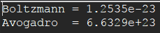 An estimate for Boltzmann’s Constant and Avogadro’s Number using data from all 10 trials of the experiment
Not bad, eh? But how exactly did the radial displacements from Brownian movement lead to this constant?
Magic?
Not quite. It’s a bit more complex than that. We first find the diffusion constant with our data in order to approximate the Boltzmann constant and finally predict Avogadro’s constant.
Einstein’s relation equation states:  where t is the time between movements, σ2 is the variance of random movements, and D is the diffusion constant we are looking for.
Thankfully, we found the random variance of movements by observing the displacements of the polystyrene beads undergoing Brownian motion which can be boiled down to the following equation: 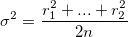 r2n represents radial displacement and is approximated from the 2-dimensional X and Y movement of the beads.
From there, we have the means to calculate the Diffusion constant, D. After that, we can calculate the Boltzmann constant with the Stokes-Einstein relation describing a particle in a viscous solution:  where k is the Boltzmann constant. T (absolute temperature), η (viscosity of water), and ρ (radius of a polystyrene bead) are all assumed to be constants measured at the beginning of the experiment.
Finally, we can relate the Boltzmann constant to Avogadro’s constant:  from the Ideal Gas Law. There we have it! Our estimate for Avogadro’s constant came out to be approximately 10% off the actual value. Not bad for some video analysis of light.
This assignment was created by David Botstein, Tamara Broderick, Ed Davisson, Daniel Marlow, William Ryu, and Kevin Wayne of Princeton University in 2005 and was personally completed in Spring 2017. Standard libraries from the course were also involved in the making of this project.